CCIM Connections
The Official Publication of The CCIM Institute
Image

Image

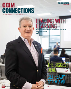
Spring 2025 Connections
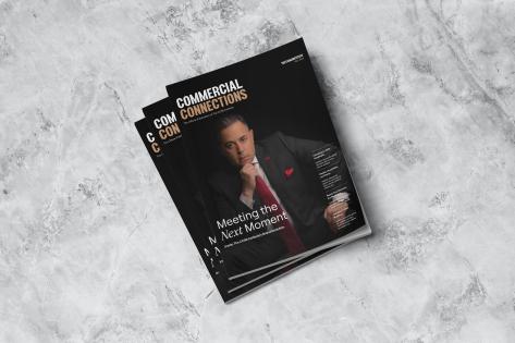
From Student to Leader
Steve Rich’s Journey to Global President and his Vision for The CCIM Institute
Read Article
The Latest Trending Articles
-
Image
 Summer 2024
President's Desk
-
Image

-
Image

-
Image
 Summer 2024
New Commercial Real Estate Certificate Program
-
Image
-
Image

-
Image
 Summer 2024
DEAL MAKERS: Summer 2024
-
Image

Image
Become a Member to Receive the Quarterly Print Issues
Also, get complimentary online access to the magazine and companion podcast.
Featured Articles by Issue
Stay Up to Date on All Issues
Hero image
Intro Text
FROM ENVIRONMENTAL SCIENTIST TO LAND SALES, GONZALEZ FOUND A SECOND CAREER IN COMMERCIAL REAL ESTATE.
Intro Text
CCIM Designees are traversing the world to make deals happen.
Hero image
Intro Text
Did we get to see you in-person in 2023?
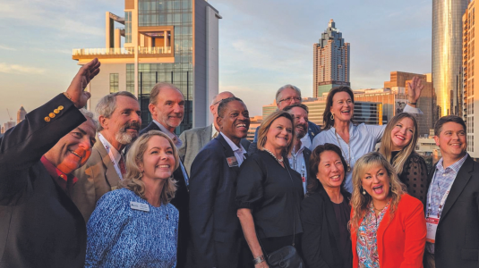
Intro Text
A glimpse into the experiences of two out of the 166 new Designees who were pinned in April 2024.