CCIM Digital Connections
The Official Publication of The CCIM Institute
Image

Image

The Latest Trending Articles
-
Image
 Summer 2024
President's Desk
-
Image

-
Image

-
Image
 Summer 2024
New Commercial Real Estate Certificate Program
-
Image
-
Image

-
Image
 Summer 2024
DEAL MAKERS: Summer 2024
-
Image

Featured Articles by Issue
Stay Up to Date on All Issues
Hero image
Intro Text
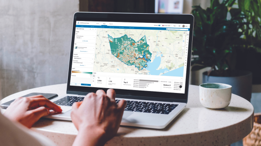
Site To Do Business is commercial real estate's most advanced digital toolkit providing essential data components and marketing tools to give your audience a broader perspective on today's market. By integrating quality online data into a dynamic mapping environment, Site To Do Business provides access to technologies and databases that wins business.
Intro Text
Driving The CCIM Institute's Growth
Hero image

Intro Text
In response to industry needs, The CCIM Institute launches a new program.
Hero image

Intro Text
Making Deals - Spring 2024